Chapter 2 Bayesian Inference

This chapter is focused on the continuous version of Bayes’ rule and how to use it in a conjugate family. The RU-486 example will allow us to discuss Bayesian modeling in a concrete way. It also leads naturally to a Bayesian analysis without conjugacy. For the non-conjugate case, there is usually no simple mathematical expression, and one must resort to computation. Finally, we discuss credible intervals, i.e., the Bayesian analog of frequentist confidence intervals, and Bayesian estimation and prediction.

It is assumed that the readers have mastered the concept of conditional probability and the Bayes’ rule for discrete random variables. Calculus is not required for this chapter; however, for those who do, we shall briefly look at an integral.

2.1 Continuous Variables and Eliciting Probability Distributions

We are going to introduce continuous variables and how to elicit probability distributions, from a prior belief to a posterior distribution using the Bayesian framework.

2.1.1 From the Discrete to the Continuous

This section leads the reader from the discrete random variable to continuous random variables. Let’s start with the binomial random variable such as the number of heads in ten coin tosses, can only take a discrete number of values: 0, 1, 2, up to 10.

When the probability of a coin landing heads is \(p\), the chance of getting \(k\) heads in \(n\) tosses is

\[P(X = k) = \left( \begin{array}{c} n \\ k \end{array} \right) p^k (1-p)^{n-k}\].

This formula is called the probability mass function (pmf) for the binomial.

The probability mass function can be visualized as a histogram in Figure 2.1. The area under the histogram is one, and the area of each bar is the probability of seeing a binomial random variable, whose value is equal to the x-value at the center of the bars base.

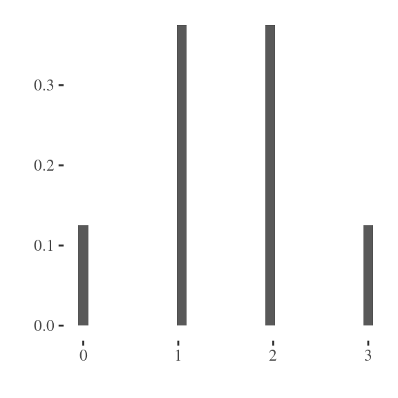
Figure 2.1: Histogram of binomial random variable

In contrast, the normal distribution, a.k.a. Gaussian distribution or the bell-shaped curve, can take any numerical value in \((-\infty,+\infty)\). A random variable generated from a normal distribution because it can take a continuum of values.

In general, if the set of possible values a random variable can take are separated points, it is a discrete random variable. But if it can take any value in some (possibly infinite) interval, then it is a continuous random variable.

When the random variable is discrete, it has a probability mass function or pmf. That pmf tells us the probability that the random variable takes each of the possible values. But when the random variable is continuous, it has probability zero of taking any single value. (Hence probability zero does not equal to impossible, an event of probabilty zero can still happen.)

We can only talk about the probability of a continuous random variable lined within some interval. For example, suppose that heights are approximately normally distributed. The probability of finding someone who is exactly 6 feet and 0.0000 inches tall (for an infinite number of 0s after the decimal point) is 0. But we can easily calculate the probability of finding someone who is between 5’11” inches tall and 6’1” inches tall.

A continuous random variable has a probability density function or pdf, instead of probability mass functions. The probability of finding someone whose height lies between 5’11” (71 inches) and 6’1” (73 inches) is the area under the pdf curve for height between those two values, as shown in the blue area of Figure 2.2.

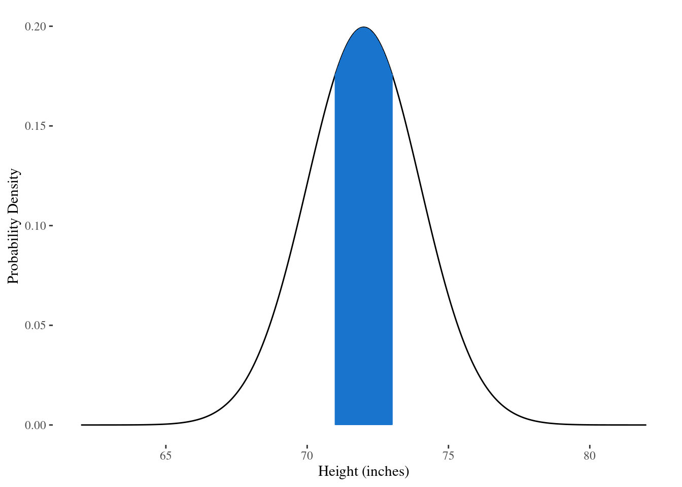
Figure 2.2: Area under curve for the probability density function

For example, a normal distribution with mean \(\mu\) and standard deviation \(\sigma\) (i.e., variance \(\sigma^2\)) is defined as

\[f(x) = \frac{1}{\sqrt{2 \pi \sigma^2}} \exp[-\frac{1}{2\sigma^2}(x-\mu)^2],\]

where \(x\) is any value the random variable \(X\) can take. This is denoted as \(X \sim N(\mu,\sigma^2)\), where \(\mu\) and \(\sigma^2\) are the parameters of the normal distribution.

Recall that a probability mass function assigns the probability that a random variable takes a specific value for the discrete set of possible values. The sum of those probabilities over all possible values must equal one.

Similarly, a probability density function is any \(f(x)\) that is non-negative and has area one underneath its curve. The pdf can be regarded as the limit of histograms made from its sample data. As the sample size becomes infinitely large, the bin width of the histogram shrinks to zero.

There are infinite number of pmf’s and an infinite number of pdf’s. Some distributions are so important that they have been given names:

• Continuous: normal, uniform, beta, gamma

• Discrete: binomial, Poisson

Here is a summary of the key ideas in this section:

1. Continuous random variables exist and they can take any value within some possibly infinite range.

2. The probability that a continuous random variable takes a specific value is zero.

3. Probabilities from a continuous random variable are determined by the density function with this non-negative and the area beneath it is one.

4. We can find the probability that a random variable lies between two values (\(c\) and \(d\)) as the area under the density function that lies between them.

2.1.2 Elicitation

Next, we introduce the concept of prior elicitation in Bayesian statistics. Often, one has a belief about the distribution of one’s data. You may think that your data come from a binomial distribution and in that case you typically know the \(n\), the number of trials but you usually do not know \(p\), the probability of success. Or you may think that your data come from a normal distribution. But you do not know the mean \(\mu\) or the standard deviation \(\sigma\) of the normal. Beside to knowing the distribution of one’s data, you may also have beliefs about the unknown \(p\) in the binomial or the unknown mean \(\mu\) in the normal.

Bayesians express their belief in terms of personal probabilities. These personal probabilities encapsulate everything a Bayesian knows or believes about the problem. But these beliefs must obey the laws of probability, and be consistent with everything else the Bayesian knows.

::: {.example #200percent} You cannot say that your probability of passing this course is 200%, no matter how confident you are. A probability value must be between zero and one. (If you still think you have a probability of 200% to pass the course, you are definitely not going to pass it.) :::

Example 2.1 You may know nothing at all about the value of \(p\) that generated some binomial data. In which case any value between zero and one is equally likely, you may want to make an inference on the proportion of people who would buy a new band of toothpaste. If you have industry experience, you may have a strong belief about the value of \(p\), but if you are new to the industry you would do nothing about \(p\). In any value between zero and one seems equally like a deal. This major personal probability is the uniform distribution whose probably density function is flat, denoted as \(\text{Unif}(0,1)\).

Example 2.2 If you were tossing a coin, most people believed that the probability of heads is pretty close to half. They know that some coins are biased and that some coins may have two heads or two tails. And they probably also know that coins are not perfectly balanced. Nonetheless, before they start to collect data by tossing the coin and counting the number of heads their belief is that values of \(p\) near 0.5 are very likely, whereas values of \(p\) near 0 or 1 are very unlikely.

Example 2.3 In real life, here are two ways to elicit a probability that you cousin will get married. A frequentist might go to the U.S. Census records and determine what proportion of people get married (or, better, what proportion of people of your cousin’s ethnicity, education level, religion, and age cohort are married). In contrast, a Bayesian might think “My cousin is brilliant, attractive, and fun. The probability that my cousin gets married is really high – probably around 0.97.”

So a Bayesian will seek to express their belief about the value of \(p\) through a probability distribution, and a very flexible family of distributions for this purpose is the beta family. A member of the beta family is specified by two parameters, \(\alpha\) and \(\beta\); we denote this as \(p \sim \text{beta}(\alpha, \beta)\). The probability density function is

\[\begin{equation} f(p) = \frac{\Gamma(\alpha+\beta)}{\Gamma(\alpha)\Gamma(\beta)} p^{\alpha-1} (1-p)^{\beta-1}, \tag{2.1} \end{equation}\] where \(0 \leq p \leq 1, \alpha>0, \beta>0\), and \(\Gamma\) is a factorial:

\[\Gamma(n) = (n-1)! = (n-1) \times (n-2) \times \cdots \times 1\]

When \(\alpha=\beta=1\), the beta distribution becomes a uniform distribution, i.e. the probabilty density function is a flat line. In other words, the uniform distribution is a special case of the beta family.

The expected value of \(p\) is \(\frac{\alpha}{\alpha+\beta}\), so \(\alpha\) can be regarded as the prior number of successes, and \(\beta\) the prior number of failures. When \(\alpha=\beta\), then one gets a symmetrical pdf around 0.5. For large but equal values of \(\alpha\) and \(\beta\), the area under the beta probability density near 0.5 is very large. Figure 2.3 compares the beta distribution with different parameter values.

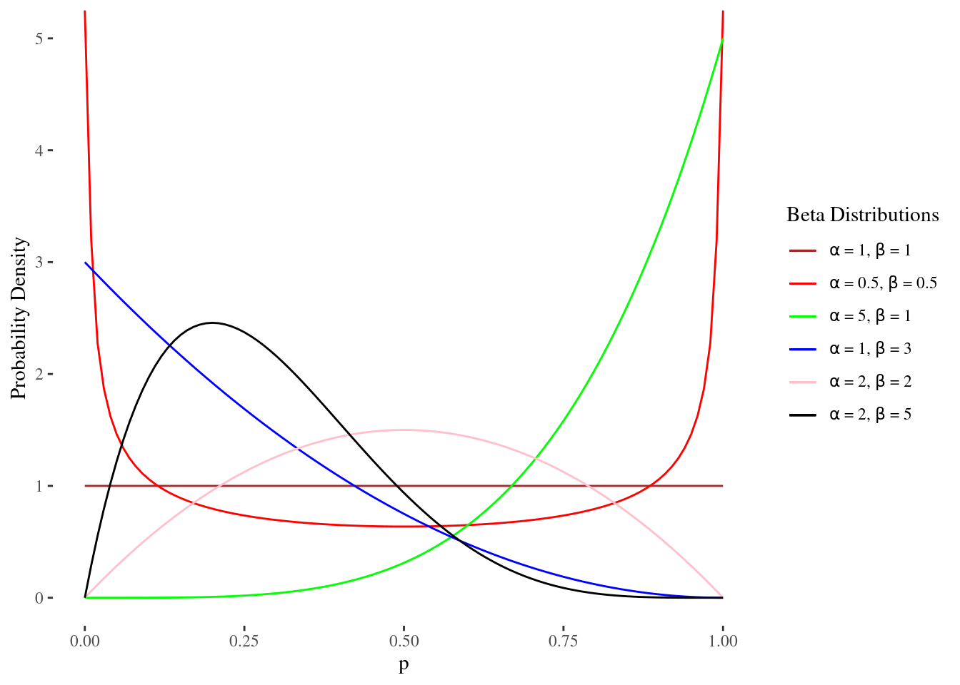
Figure 2.3: Beta family

These kinds of priors are probably appropriate if you want to infer the probability of getting heads in a coin toss. The beta family also includes skewed densities, which is appropriate if you think that \(p\) the probability of success in ths binomial trial is close to zero or one.

Bayes’ rule is a machine to turn one’s prior beliefs into posterior beliefs. With binomial data you start with whatever beliefs you may have about \(p\), then you observe data in the form of the number of head, say 20 tosses of a coin with 15 heads.

Next, Bayes’ rule tells you how the data changes your opinion about \(p\). The same principle applies to all other inferences. You start with your prior probability distribution over some parameter, then you use data to update that distribution to become the posterior distribution that expresses your new belief.

These rules ensure that the change in distributions from prior to posterior is the uniquely rational solution. So, as long as you begin with the prior distribution that reflects your true opinion, you can hardly go wrong.

However, expressing that prior can be difficult. There are proofs and methods whereby a rational and coherent thinker can self-illicit their true prior distribution, but these are impractical and people are rarely rational and coherent.

The good news is that with the few simple conditions no matter what part distribution you choose. If enough data are observed, you will converge to an accurate posterior distribution. So, two bayesians, say the reference Thomas Bayes and the agnostic Ajay Good can start with different priors but, observe the same data. As the amount of data increases, they will converge to the same posterior distribution.

Here is a summary of the key ideas in this section:

1. Bayesians express their uncertainty through probability distributions.

2. One can think about the situation and self-elicit a probability distribution that approximately reflects his/her personal probability.

3. One’s personal probability should change according Bayes’ rule, as new data are observed.

4. The beta family of distribution can describe a wide range of prior beliefs.

2.1.3 Conjugacy

Next, let’s introduce the concept of conjugacy in Bayesian statistics.

Suppose we have the prior beliefs about the data as below:

• Binomial distribution \(\text{Bin}(n,p)\) with \(n\) known and \(p\) unknown

• Prior belief about \(p\) is \(\text{beta}(\alpha,\beta)\)

Then we observe \(x\) success in \(n\) trials, and it turns out the Bayes’ rule implies that our new belief about the probability density of \(p\) is also the beta distribution, but with different parameters. In mathematical terms,

\[\begin{equation} p|x \sim \text{beta}(\alpha+x, \beta+n-x). \tag{2.2} \end{equation}\]

This is an example of conjugacy. Conjugacy occurs when the posterior distribution is in the same family of probability density functions as the prior belief, but with new parameter values, which have been updated to reflect what we have learned from the data.

Why are the beta binomial families conjugate? Here is a mathematical explanation.

Recall the discrete form of the Bayes’ rule:

\[P(A_i|B) = \frac{P(B|A_i)P(A_i)}{\sum^n_{j=1}P(B|A_j)P(A_j)}\]

However, this formula does not apply to continuous random variables, such as the \(p\) which follows a beta distribution, because the denominator sums over all possible values (must be finitely many) of the random variable.

But the good news is that the \(p\) has a finite range – it can take any value only between 0 and 1. Hence we can perform integration, which is a generalization of the summation. The Bayes’ rule can also be written in continuous form as:

\[\pi^*(p|x) = \frac{P(x|p)\pi(p)}{\int^1_0 P(x|p)\pi(p) dp}.\]

This is analogus to the discrete form, since the integral in the denominator will also be equal to some constant, just like a summation. This constant ensures that the total area under the curve, i.e. the posterior density function, equals 1.

Note that in the numerator, the first term, \(P(x|p)\), is the data likelihood – the probability of observing the data given a specific value of \(p\). The second term, \(\pi(p)\), is the probability density function that reflects the prior belief about \(p\).

In the beta-binomial case, we have \(P(x|p)=\text{Bin}(n,p)\) and \(\pi(p)=\text{beta}(\alpha,\beta)\).

Plugging in these distributions, we get

\[\begin{aligned} \pi^*(p|x) &= \frac{1}{\text{some number}} \times P(x|p)\pi(p) \\ &= \frac{1}{\text{some number}} [\left( \begin{array}{c} n \\ x \end{array} \right) p^x (1-p)^{n-x}] [\frac{\Gamma(\alpha+\beta)}{\Gamma(\alpha)\Gamma(\beta)} p^{\alpha-1} (1-p)^{\beta-1}] \\ &= \frac{\Gamma(\alpha+\beta+n)}{\Gamma(\alpha+x)\Gamma(\beta+n-x)} \times p^{\alpha+x-1} (1-p)^{\beta+n-x-1} \end{aligned}\]

Let \(\alpha^* = \alpha + x\) and \(\beta^* = \beta+n-x\), and we get

\[\pi^*(p|x) = \text{beta}(\alpha^*,\beta^*) = \text{beta}(\alpha+x, \beta+n-x),\]

same as the posterior formula in Equation (2.2).

We can recognize the posterior distribution from the numerator \(p^{\alpha+x-1}\) and \((1-p)^{\beta+n-x-1}\). Everything else are just constants, and they must take the unique value, which is needed to ensure that the area under the curve between 0 and 1 equals 1. So they have to take the values of the beta, which has parameters \(\alpha+x\) and \(\beta+n-x\).

This is a cute trick. We can find the answer without doing the integral simply by looking at the form of the numerator.

Without conjugacy, one has to do the integral. Often, the integral is impossible to evaluate. That obstacle is the primary reason that most statistical theory in the 20th century was not Bayesian. The situation did not change until modern computing allowed researchers to compute integrals numerically.

In summary, some pairs of distributions are conjugate. If your prior is in one and your data comes from the other, then your posterior is in the same family as the prior, but with new parameters. We explored this in the context of the beta-binomial conjugate families. And we saw that conjugacy meant that we could apply the continuous version of Bayes’ rule without having to do any integration.

2.2 Three Conjugate Families

In this section, the three conjugate families are beta-binomial, gamma-Poisson, and normal-normal pairs. Each of them has its own applications in everyday life.

2.2.1 Inference on a Binomial Proportion

Example 2.4 Recall Example 1.8, a simplified version of a real clinical trial taken in Scotland. It concerned RU-486, a morning after pill that was being studied to determine whether it was effective at preventing unwanted pregnancies. It had 800 women, each of whom had intercourse no more than 72 hours before reporting to a family planning clinic to seek contraception.

Half of these women were randomly assigned to the standard contraceptive, a large dose of estrogen and progesterone. And half of the women were assigned RU-486. Among the RU-486 group, there were no pregnancies. Among those receiving the standard therapy, four became pregnant.

Statistically, one can model these data as coming from a binomial distribution. Imagine a coin with two sides. One side is labeled standard therapy and the other is labeled RU-486. The coin was tossed four times, and each time it landed with the standard therapy side face up.

A frequentist would analyze the problem as below:

• The parameter \(p\) is the probability of a preganancy comes from the standard treatment.

• \(H_0: p \geq 0.5\) and \(H_A: p < 0.5\)

• The p-value is \(0.5^4 = 0.0625 > 0.05\)

Therefore, the frequentist fails to reject the null hypothesis, and will not conclude that RU-486 is superior to standard therapy.

Remark: The significance probability, or p-value, is the chance of observing data that are as or more supportive of the alternative hypothesis than the data that were collected, when the null hypothesis is true.

Now suppose a Bayesian performed the analysis. She may set her beliefs about the drug and decide that she has no prior knowledge about the efficacy of RU-486 at all. This would be reasonable if, for example, it were the first clinical trial of the drug. In that case, she would be using the uniform distribution on the interval from 0 to 1, which corresponds to the \(\text{beta}(1,1)\) density. In mathematical terms,

\[p \sim \text{Unif}(0,1) = \text{beta}(1,1).\]

From conjugacy, we know that since there were four failures for RU-486 and no successes, that her posterior probability of an RU-486 child is

\[p|x \sim \text{beta}(1+0,1+4) = \text{beta}(1,5).\]

This is a beta that has much more area near \(p\) equal to 0. The mean of \(\text{beta}(\alpha,\beta)\) is \(\frac{\alpha}{\alpha+\beta}\). So this Bayesian now believes that the unknown \(p\), the probability of an RU-468 child, is about 1 over 6.

The standard deviation of a beta distribution with parameters in alpha and beta also has a closed form:

\[p \sim \text{beta}(\alpha,\beta) \Rightarrow \text{Standard deviation} = \sqrt{\frac{\alpha\beta}{(\alpha+\beta)^2(\alpha+\beta+1)}}\]

Before she saw the data, the Bayesian’s uncertainty expressed by her standard deviation was 0.71. After seeing the data, it was much reduced – her posterior standard deviation is just 0.13.

We promised not to do much calculus, so I hope you will trust me to tell you that this Bayesian now believes that her posterior probability that \(p < 0.5\) is 0.96875. She thought there was a 50-50 chance that RU-486 is better. But now she thinks there is about a 97% chance that RU-486 is better.

Suppose a fifth child were born, also to a mother who received standard chip therapy. Now the Bayesian’s prior is beta(1, 5) and the additional data point further updates her to a new posterior beta of 1 and 6. As data comes in, the Bayesian’s previous posterior becomes her new prior, so learning is self-consistent.

This example has taught us several things:

1. We saw how to build a statistical model for an applied problem.

2. We could compare the frequentist and Bayesian approaches to inference and see large differences in the conclusions.

3. We saw how the data changed the Bayesian’s opinion with a new mean for p and less uncertainty.

4. We learned that Bayesian’s continually update as new data arrive. Yesterday’s posterior is today’s prior.

2.2.2 The Gamma-Poisson Conjugate Families

A second important case is the gamma-Poisson conjugate families. In this case the data come from a Poisson distribution, and the prior and posterior are both gamma distributions.

The Poisson random variable can take any non-negative integer value all the way up to infinity. It is used in describing count data, where one counts the number of independent events that occur in a fixed amount of time, a fixed area, or a fixed volume.

Moreover, the Poisson distribution has been used to describe the number of phone calls one receives in an hour. Or, the number of pediatric cancer cases in the city, for example, to see if pollution has elevated the cancer rate above that of in previous years or for similar cities. It is also used in medical screening for diseases, such as HIV, where one can count the number of T-cells in the tissue sample.

The Poisson distribution has a single parameter \(\lambda\), and it is denoted as \(X \sim \text{Pois}(\lambda)\) with \(\lambda>0\). The probability mass function is

\[P(X=k) = \frac{\lambda^k}{k!} e^{-\lambda} \text{ for } k=0,1,\cdots,\]

where \(k! = k \times (k-1) \times \cdots \times 1\). This gives the probability of observing a random variable equal to \(k\).

Note that \(\lambda\) is both the mean and the variance of the Poisson random variable. It is obvious that \(\lambda\) must be greater than zero, because it represents the mean number of counts, and the variance should be greater than zero (except for constants, which have zero variance).

Example 2.5 Famously, von Bortkiewicz used the Poisson distribution to study the number of Prussian cavalrymen who were kicked to death by a horse each year. This is count data over the course of a year, and the events are probably independent, so the Poisson model makes sense.

He had data on 15 cavalry units for the 20 years between 1875 and 1894, inclusive. The total number of cavalrymen who died by horse kick was 200.

One can imagine that a Prussian general might want to estimate \(\lambda\). The average number per year, per unit. Perhaps in order to see whether some educational campaign about best practices for equine safety would make a difference.

Suppose the Prussian general is a Bayesian. Introspective elicitation leads him to think that \(\lambda=0.75\) and standard deviation 1.

Modern computing was unavailable at that time yet, so the Prussian general will need to express his prior as a member of a family conjugate to the Poisson. It turns out that this family consists of the gamma distributions. Gamma distributions describe continuous non-negative random variables. As we know, the value of \(\lambda\) in the Poisson can take any non-negative value so this fits.

The gamma family is flexible, and Figure 2.4 illustrates a wide range of gamma shapes.

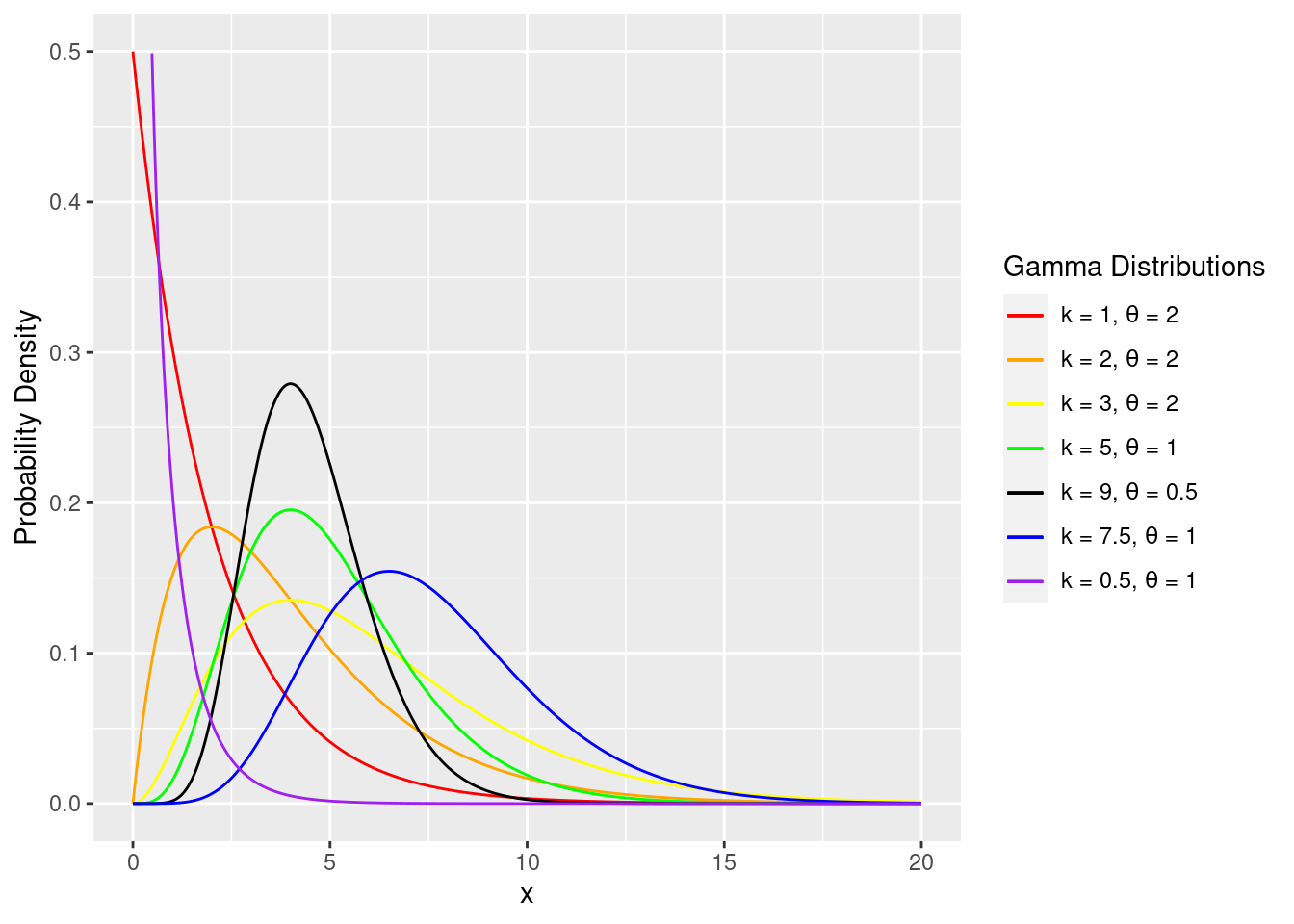
Figure 2.4: Gamma family

The probability density function for the gamma is indexed by shape \(k\) and scale \(\theta\), denoted as \(\text{Gamma}(k,\theta)\) with \(k,\theta > 0\). The mathematical form of the density is

\[\begin{equation} f(x) = \dfrac{1}{\Gamma(k)\theta^k} x^{k-1} e^{-x/\theta} \tag{2.3} \end{equation}\] where

\[\begin{equation} \Gamma(z) = \int^{\infty}_0 x^{z-1} e^{-x} dx. \tag{2.4} \end{equation}\] \(\Gamma(z)\), the gamma function, is simply a constant that ensures the area under curve between 0 and 1 sums to 1, just like in the beta probability distribution case of Equation (2.1). A special case is that \(\Gamma(n) = (n-1)!\) when \(n\) is a positive integer.

However, some books parameterize the gamma distribution in a slightly different way with shape \(\alpha = k\) and rate (inverse scale) \(\beta=1/\theta\):

\[f(x) = \frac{\beta^{\alpha}}{\Gamma(\alpha)} x^{\alpha-1} e^{-\beta x}\]

For this example, we use the \(k\)-\(\theta\) parameterization, but you should always check which parameterization is being used. For example, \(\mathsf{R}\) uses the \(\alpha\)-\(\beta\) parameterization by default.
In the the later material we find that using the rate parameterization is more convenient.

For our parameterization, the mean of \(\text{Gamma}(k,\theta)\) is \(k\theta\), and the variance is \(k\theta^2\). We can get the general’s prior as below:

\[\begin{aligned} \text{Mean} &= k\theta = 0.75 \\ \text{Standard deviation} &= \theta\sqrt{k} = 1 \end{aligned}\]

Hence \[k = \frac{9}{16} \text{ and } \theta = \frac{4}{3}\]

For the gamma Poisson conjugate family, suppose we observed data \(x_1, x_2, \cdots, x_n\) that follow a Poisson distribution.Then similar to the previous section, we would recognize the kernel of the gamma when using the gamma-Poisson family. The posterior \(\text{Gamma}(k^*, \theta^*)\) has parameters

\[k^* = k + \sum^n_{i=1} x_i \text{ and } \theta^* = \frac{\theta}{(n\theta+1)}.\]

For this dataset, \(N = 15 \times 20 = 300\) observations, and the number of casualities is 200. Therefore, the general now thinks that the average number of Prussian cavalry officers who die at the hoofs of their horses follows a gamma distribution with the parameters below:

\[\begin{aligned} k^* &= k + \sum^n_{i=1} x_i = \frac{9}{16} + 200 = 200.5625 \\ \theta^* = \frac{\theta}{(n\theta+1)} &= \frac{4/3}{300\times(4/3)} = 0.0033 \end{aligned}\]

How the general has changed his mind is described in Table 2.1. After seeing the data, his uncertainty about lambda, expressed as a standard deviation, shrunk from 1 to 0.047.

Table 2.1: Before and after seeing the data

	lambda	Standard Deviation
Before	0.75	1.000
After	0.67	0.047

In summary, we learned about the Poisson and gamma distributions; we also knew that the gamma-Poisson families are conjugate. Moreover, we learned the updating fomula, and applied it to a classical dataset.

2.2.3 The Normal-Normal Conjugate Families

There are other conjugate families, and one is the normal-normal pair. If your data come from a normal distribution with known variance \(\sigma^2\) but unknown mean \(\mu\), and if your prior on the mean \(\mu\), has a normal distribution with self-elicited mean \(\nu\) and self-elicited variance \(\tau^2\), then your posterior density for the mean, after seeing a sample of size \(n\) with sample mean \(\bar{x}\), is also normal. In mathematical notation, we have

\[\begin{aligned} x|\mu &\sim N(\mu,\sigma^2) \\ \mu &\sim N(\nu, \tau^2) \end{aligned}\]

As a practical matter, one often does not know \(\sigma^2\), the standard deviation of the normal from which the data come. In that case, you could use a more advanced conjugate family that we will describe in 4.1. But there are cases in which it is reasonable to treat the \(\sigma^2\) as known.

Example 2.6 An analytical chemist whose balance produces measurements that are normally distributed with mean equal to the true mass of the sample and standard deviation that has been estimated by the manufacturer balance and confirmed against calibration standards provided by the National Institute of Standards and Technology.

Note that this normal-normal assumption made by the anayltical chemist is technically wrong, but still reasonable.

1. The normal family puts some probability on all possible values between \((-\infty,+\infty)\). But the mass on the balance can never be negative. However, the normal prior on the unknown mass is usually so concentrated on positive values that the normal distribution is still a good approximation.

2. Even if the chemist has repeatedly calibrated her balance with standards from the National Institute of Standards and Technology, she still will not know its standard deviation precisely. However, if she has done it often and well, it is probably a sufficiently good approximation to assume that the standard deviation is known.

For the normal-normal conjugate families, assume the prior on the unknown mean follows a normal distribution, i.e. \(\mu \sim N(\nu, \tau^2)\). We also assume that the data \(x_1,x_2,\cdots,x_n\) are independent and come from a normal with variance \(\sigma^2\).

Then the posterior distribution of \(\mu\) is also normal, with mean as a weighted average of the prior mean and the sample mean. We have

\[\mu|x_1,x_2,\cdots,x_n \sim N(\nu^*, \tau^{*2}),\]

where

\[\nu^* = \frac{\nu\sigma^2 + n\bar{x}\tau^2}{\sigma^2 + n\tau^2} \text{ and } \tau^* = \sqrt{\frac{\sigma^2\tau^2}{\sigma^2 + n\tau^2}}.\]

Let’s continue from Example 2.6, and suppose she wants to measure the mass of a sample of ammonium nitrate.

Her balance has a known standard deviation of 0.2 milligrams. By looking at the sample, she thinks this mass is about 10 milligrams and based on her previous experience in estimating masses, her guess has the standard deviation of 2. So she decides that her prior for the mass of the sample is a normal distribution with mean, 10 milligrams, and standard deviation, 2 milligrams.

Now she collects five measurements on the sample and finds that the average of those is 10.5. By conjugacy of the normal-normal family, our posterior belief about the mass of the sample has the normal distribution.

The new mean of that posterior normal is found by plugging into the formula:

\[\begin{aligned} \mu &\sim N(\nu=10, \tau^2=2^2) \\ \nu^* &= \frac{\nu\sigma^2 + n\bar{x}\tau^2}{\sigma^2 + n\tau^2} = \frac{10\times(0.2)^2+5\times10.5\times2^2}{(0.2)^2+5\times2^2} = 10.499\\ \tau^* &= \sqrt{\frac{\sigma^2\tau^2}{\sigma^2 + n\tau^2}} = \sqrt{(0.2)^2\times2^2}{(0.2)^2+5\times2^2} = 0.089. \end{aligned}\]

Before seeing the data, the Bayesian analytical chemist thinks the ammonium nitrate has mass 10 mg and uncertainty (standard deviation) 2 mg. After seeing the data, she thinks the mass is 10.499 mg and standard deviation 0.089 mg. Her posterior mean has shifted quite a bit and her uncertainty has dropped by a lot. That’s exactly what an analytical chemist wants.

This is the last of the three examples of conjugate families. There are many more, but they do not suffice for every situation one might have.

We learned several things in this lecture. First, we learned the new pair of conjugate families and the relevant updating formula. Also, we worked a realistic example problem that can arise in practical situations.

2.3 Credible Intervals and Predictive Inference

In this part, we are going to quantify the uncertainty of the parameter by credible intervals after incorporating the data. Then we can use predictive inference to identify the posterior distribution for a new random variable.

2.3.1 Non-Conjugate Priors

In many applications, a Bayesian may not be able to use a conjugate prior. Sometimes she may want to use a reference prior, which injects the minimum amount of personal belief into the analysis. But most often, a Bayesian will have a personal belief about the problem that cannot be expressed in terms of a convenient conjugate prior.

For example, we shall reconsider the RU-486 case from earlier in which four children were born to standard therapy mothers. But no children were born to RU-486 mothers. This time, the Bayesian believes that the probability p of an RU-486 baby is uniformly distributed between 0 and one-half, but has a point mass of 0.5 at one-half. That is, she believes there is a 50% chance that no difference exists between standard therapy and RU-486. But if a difference exists, she thinks that RU-486 is better, but she is completely unsure about how much better it would be.

In mathematical notation, the probability density function of \(p\) is

\[\pi(p) = \left\{ \begin{array}{ccc} 1 & \text{for} & 0 \leq p < 0.5 \\ 0.5 & \text{for} & p = 0.5 \\ 0 & \text{for} & p < 0 \text{ or } p > 0.5 \end{array}\right.\]

We can check that the area under the density curve, plus the amount of the point mass, equals 1.

The cumulative distribution function, \(P(p\leq x)\) or \(F(x)\), is

\[P(p \leq x) = F(x) = \left\{ \begin{array}{ccc} 0 & \text{for} & x < 0 \\ x & \text{for} & 0 \leq x < 0.5 \\ 1 & \text{for} & x \geq 0.5 \end{array}\right.\]

Why would this be a reasonable prior for an analyst to self-elicit? One reason is that in clinical trials, there is actually quite a lot of preceding research on the efficacy of the drug. This research might be based on animal studies or knowledge of the chemical activity of the molecule. So the Bayesian might feel sure that there is no possibility that RU-486 is worse than the standard treatment. And her interest is on whether the therapies are equivalent and if not, how much better RU-486 is than the standard therapy.

As previously mentioned, the posterior distribution \(\pi^*(p)\) for \(p\) has a complex mathematical form. That is why Bayesian inference languished for so many decades until computational power enabled numerical solutions. But now we have simulation tools to help us, and one of them is called JAGS (Just Another Gibbs Sampler).

If we apply JAGS to the RU-486 data with this non-conjugate prior, we can find the posterior distribution \(\pi^*(p)\), as in Figure 2.5. At a high level, this program is defining the binomial probability, that is the likelihood of seeing 0 RU-486 children, which is binomial. And then it defines the prior by using a few tricks to draw from either a uniform on the interval from 0 to one-half, or else draw from the point mass at one-half. Then it calls the JAGS model function, and draws 5,000 times from the posterior and creates a histogram of the results.

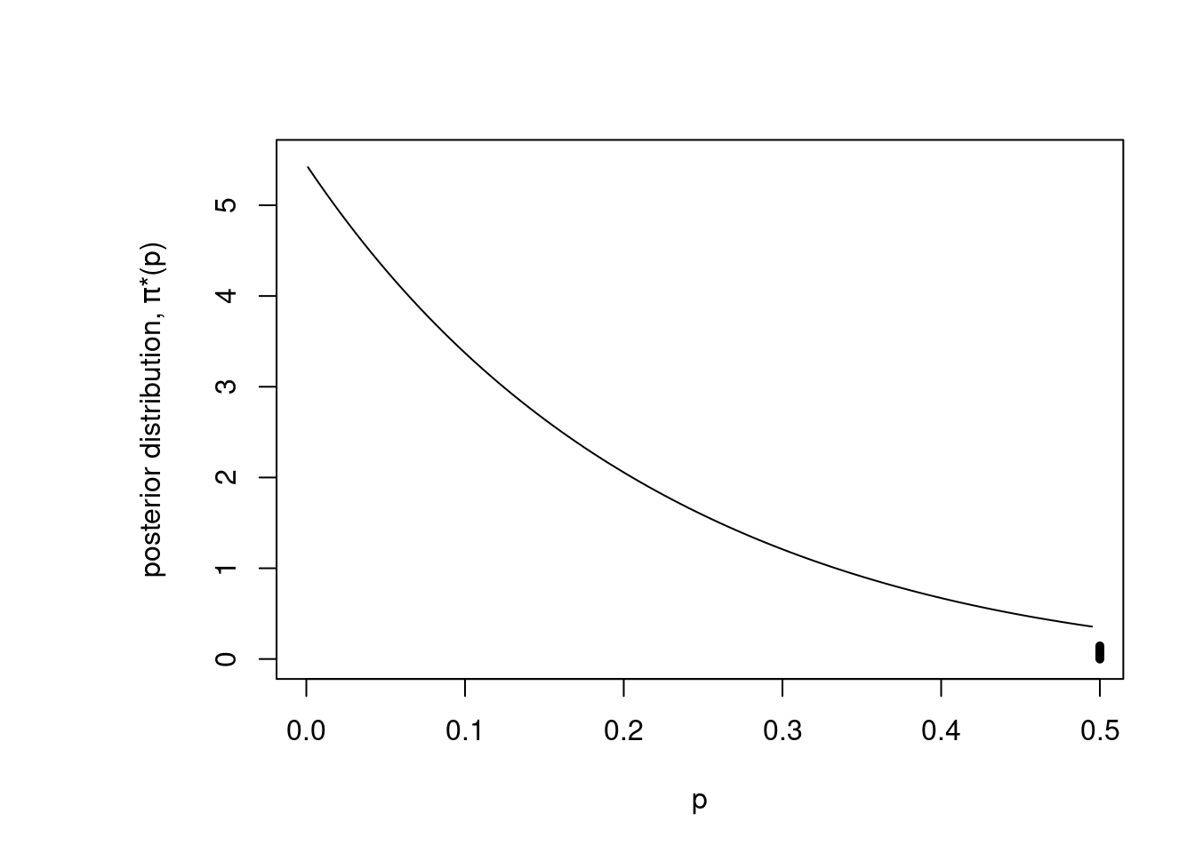
Figure 2.5: Posterior with JAGS

The posterior distribution is decreasing when \(p\) is between 0 and 0.5, and has a point mass of probability at 0.5. But now the point mass has less weights than before. Also, note that the data have changed the posterior away from the original uniform prior when \(p\) is between 0 and 0.5. The analyst sees a lot of probability under the curve near 0, which responds to the fact that no children were born to RU-486 mothers.

This section is mostly a look-ahead to future material. We have seen that a Bayesian might reasonably employ a non-conjugate prior in a practical application. But then she will need to employ some kind of numerical computation to approximate the posterior distribution. Additionally, we have used a computational tool, JAGS, to approximate the posterior for \(p\), and identified its three important elements, the probability of the data given \(p\), that is the likelihood, and the prior, and the call to the Gibbs sampler.

2.3.2 Credible Intervals

In this section, we introduce credible intervals, the Bayesian alternative to confidence intervals. Let’s start with the confidence intervals, which are the frequentist way to express uncertainty about an estimate of a population mean, a population proportion or some other parameter.

A confidence interval has the form of an upper and lower bound.

\[L, U = \text{pe} \pm \text{se} \times \text{cv}\]

where \(L\), \(U\) are the lower bound and upper bound of the confidence interval respectively, \(\text{pe}\) represents “point estimates”, \(\text{se}\) is the standard error, and \(\text{cv}\) is the critical value.

Most importantly, the interpretation of a 95% confidence interval on the mean is that “95% of similarly constructed intervals will contain the true mean”, not “the probability that true mean lies between \(L\) and \(U\) is 0.95”.

The reason for this frequentist wording is that a frequentist may not express his uncertainty as a probability. The true mean is either within the interval or not, so the probability is zero or one. The problem is that the frequentist does not know which is the case.

On the other hand, Bayesians have no such qualms. It is fine for us to say that “the probability that the true mean is contained within a given interval is 0.95”. To distinguish our intervals from confidence intervals, we call them credible intervals.

Recall the RU-486 example. When the analyst used the beta-binomial family, she took the prior as \(p \sim \text{beta}(1,1)\), the uniform distribution, where \(p\) is the probability of a child having a mother who received RU-486.

After we observed four children born to mothers who received conventional therapy, her posterior is \(p|x \sim \text{beta}(1,5)\). In Figure 2.6, the posterior probability density for \(\text{beta}(1,5)\) puts a lot of probability near zero and very little probability near one.

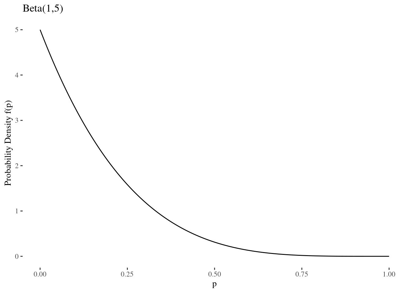
Figure 2.6: RU-486 Posterior

For the Bayesian, her 95% credible interval is just any \(L\) and \(U\) such that the posterior probability that \(L < p < U\) is \(0.95\). The shortest such interval is obviously preferable.

To find this interval, the Bayesian looks at the area under the \(\text{beta}(1,5)\) distribution, that lies to the left of a value x.

The density function of the \(\text{beta}(1,5)\) is \[f(p) = 5 (1-p)^4 \text{ for } 0 \leq p \leq 1,\]

and the cumulative distribution function, which represents the area under the density function \(f(p)\) between \(0\) and \(x\) is \[P(p\leq x)= F(x) = \int_0^x f(p)\, dp = 1 - (1-x)^5 ~\text{ for } 0 \leq p \leq 1.\]

The Bayesian can use this to find \(L, U\) with area 0.95 under the density curve between them, i.e. \(F(U) - F(L) = 0.95\). Note that the Bayesian credible interval is asymmetric, unlike the symmetric confidence intervals that frequentists often obtain. It turns out that \(L = 0\) and \(U = 0.45\) is the shortest interval with probability 0.95 of containing \(p\).

What have we done? We have seen the difference in interpretations between the frequentist confidence interval and the Bayesian credible interval. Also, we have seen the general form of a credible interval. Finally, we have done a practical example constructing a 95% credible interval for the RU-486 data set.

2.3.3 Predictive Inference

Predictive inference arises when the goal is not to find a posterior distribution over some parameter, but rather to find a posterior distribution over some random variable depends on the parameter.

Specifically, we want to make an inference on a random variable \(X\) with probability densifity function \(f(x|\theta)\), where you have some personal or prior probability distribution \(p(\theta)\) for the parameter \(\theta\).

To solve this, one needs to integrate: \[P(X \leq x) = \int^{\infty}_{-\infty} P(X \leq x | \theta)\, p(\theta)d\theta = \int_{-\infty}^\infty \left(\int_{-\infty}^x f(s|\theta)\, ds\right)p(\theta)\, d\theta\]

The equation gives us the weighted average of the probabilities for \(X\), where the weights correspond to the personal probability on \(\theta\). Here we will not perform the integral case; instead, we will illustrate the thinking with a discrete example.

Example 2.7 Suppose you have two coins. One coin has probability 0.7 of coming up heads, and the other has probability 0.4 of coming up heads. You are playing a gambling game with a friend, and you draw one of those two coins at random from a bag.

Before you start the game, your prior belief is that the probability of choosing the 0.7 coin is 0.5. This is reasonable, because both coins were equally likely to be drawn. In this game, you win if the coin comes up heads.

Suppose the game starts, you have tossed twice, and have obtained two heads. Then what is your new belief about \(p\), the probability that you are using the 0.7 coin?

This is just a simple application of the discrete form of Bayes’ rule.

• Prior: \(p=0.5\)
• Posterior: \[p^* = \frac{P(\text{2 heads}|0.7) \times 0.5}{P(\text{2 heads}|0.7) \times 0.5 + P(\text{2 heads}|0.4) \times 0.5} = 0.754.\]

However, this does not answer the important question – What is the predictive probability that the next toss will come up heads? This is of interest because you are gambling on getting heads.

Fortunately, the predictive probability of getting heads is not difficult to calculate:

• \(p^* \text{ of 0.7 coin } = 0.754\)
• \(p^* \text{ of 0.4 coin } = 1 − 0.754 = 0.246\)
• \(P(\text{heads}) = P(\text{heads} | 0.7) \times 0.754 + P(\text{heads} | 0.4) \times 0.246 = 0.626\)

Therefore, the predictive probability that the next toss will come up heads is 0.626.

Note that most realistic predictive inference problems are more complicated and require one to use integrals. For example, one might want to know the chance that a fifth child born in the RU-486 clinical trial will have a mother who received RU-486. Or you might want to know the probability that your stock broker’s next recommendation will be profitable.

We have learned three things in this section. First, often the real goal is a prediction about the value of a future random variable, rather than making an estimate of a parameter. Second, these are deep waters, and often one needs to integrate. Finally, in certain simple cases where the parameter can only take discrete values, one can find a solution without integration. In our example, the parameter could only take two values to indicate which of the two coins was being used.