Chapter 1 The Basics of Bayesian Statistics
Bayesian statistics mostly involves conditional probability, which is the the probability of an event A given event B, and it can be calculated using the Bayes rule. The concept of conditional probability is widely used in medical testing, in which false positives and false negatives may occur. A false positive can be defined as a positive outcome on a medical test when the patient does not actually have the disease they are being tested for. In other words, it’s the probability of testing positive given no disease. Similarly, a false negative can be defined as a negative outcome on a medical test when the patient does have the disease. In other words, testing negative given disease. Both indicators are critical for any medical decisions.
For how the Bayes’ rule is applied, we can set up a prior, then calculate posterior probabilities based on a prior and likelihood. That is to say, the prior probabilities are updated through an iterative process of data collection.
1.1 Bayes’ Rule
This section introduces how the Bayes’ rule is applied to calculating conditional probability, and several real-life examples are demonstrated. Finally, we compare the Bayesian and frequentist definition of probability.
1.1.1 Conditional Probabilities & Bayes’ Rule
Consider Table 1.1. It shows the results of a poll among 1,738 adult Americans. This table allows us to calculate probabilities.
| 18-29 | 30-49 | 50-64 | 65+ | Total | |
|---|---|---|---|---|---|
| Used online dating site | 60 | 86 | 58 | 21 | 225 |
| Did not use online dating site | 255 | 426 | 450 | 382 | 1513 |
| Total | 315 | 512 | 508 | 403 | 1738 |
For instance, the probability of an adult American using an online dating site can be calculated as \[\begin{multline*} P(\text{using an online dating site}) = \\ \frac{\text{Number that indicated they used an online dating site}}{\text{Total number of people in the poll}} = \frac{225}{1738} \approx 13\%. \end{multline*}\] This is the overall probability of using an online dating site. Say, we are now interested in the probability of using an online dating site if one falls in the age group 30-49. Similar to the above, we have \[\begin{multline*} P(\text{using an online dating site} \mid \text{in age group 30-49}) = \\ \frac{\text{Number in age group 30-49 that indicated they used an online dating site}}{\text{Total number in age group 30-49}} = \frac{86}{512} \approx 17\%. \end{multline*}\] Here, the pipe symbol `|’ means conditional on. This is a conditional probability as one can consider it the probability of using an online dating site conditional on being in age group 30-49.
We can rewrite this conditional probability in terms of ‘regular’ probabilities by dividing both numerator and the denominator by the total number of people in the poll. That is, \[\begin{multline*} P(\text{using an online dating site} \mid \text{in age group 30-49}) \\ \begin{split} &= \frac{\text{Number in age group 30-49 that indicated they used an online dating site}}{\text{Total number in age group 30-49}} \\ &= \frac{\frac{\text{Number in age group 30-49 that indicated they used an online dating site}}{\text{Total number of people in the poll}}}{\frac{\text{Total number in age group 30-49}}{\text{Total number of people in the poll}}} \\ &= \frac{P(\text{using an online dating site \& falling in age group 30-49})}{P(\text{Falling in age group 30-49})}. \end{split} \end{multline*}\] It turns out this relationship holds true for any conditional probability and is known as Bayes’ rule:
Definition 1.1 (Bayes' Rule) The conditional probability of the event \(A\) conditional on the event \(B\) is given by
\[ P(A \mid B) = \frac{P(A \,\&\, B)}{P(B)}. \]
Example 1.1 What is the probability that an 18-29 year old from Table 1.1 uses online dating sites?
Note that the question asks a question about 18-29 year olds. Therefore, it conditions on being 18-29 years old. Bayes’ rule provides a way to compute this conditional probability:
\[\begin{multline*} P(\text{using an online dating site} \mid \text{in age group 18-29}) \\ \begin{split} &= \frac{P(\text{using an online dating site \& falling in age group 18-29})}{P(\text{Falling in age group 18-29})} \\ &= \frac{\frac{\text{Number in age group 18-29 that indicated they used an online dating site}}{\text{Total number of people in the poll}}}{\frac{\text{Total number in age group 18-29}}{\text{Total number of people in the poll}}} \\ &= \frac{\text{Number in age group 18-29 that indicated they used an online dating site}}{\text{Total number in age group 18-29}} = \frac{60}{315} \approx 19\%. \end{split} \end{multline*}\]
1.1.2 Bayes’ Rule and Diagnostic Testing
To better understand conditional probabilities and their importance, let us consider an example involving the human immunodeficiency virus (HIV). In the early 1980s, HIV had just been discovered and was rapidly expanding. There was major concern with the safety of the blood supply. Also, virtually no cure existed making an HIV diagnosis basically a death sentence, in addition to the stigma that was attached to the disease.
These made false positives and false negatives in HIV testing highly undesirable. A false positive is when a test returns postive while the truth is negative. That would for instance be that someone without HIV is wrongly diagnosed with HIV, wrongly telling that person they are going to die and casting the stigma on them. A false negative is when a test returns negative while the truth is positive. That is when someone with HIV undergoes an HIV test which wrongly comes back negative. The latter poses a threat to the blood supply if that person is about to donate blood.
The probability of a false positive if the truth is negative is called the false positive rate. Similarly, the false negative rate is the probability of a false negative if the truth is positive. Note that both these rates are conditional probabilities: The false positive rate of an HIV test is the probability of a positive result conditional on the person tested having no HIV.
The HIV test we consider is an enzyme-linked immunosorbent assay, commonly known as an ELISA. We would like to know the probability that someone (in the early 1980s) has HIV if ELISA tests positive. For this, we need the following information. ELISA’s true positive rate (one minus the false negative rate), also referred to as sensitivity, recall, or probability of detection, is estimated as \[ P(\text{ELISA is positive} \mid \text{Person tested has HIV}) = 93\% = 0.93. \] Its true negative rate (one minus the false positive rate), also referred to as specificity, is estimated as \[ P(\text{ELISA is negative} \mid \text{Person tested has no HIV}) = 99\% = 0.99. \] Also relevant to our question is the prevalence of HIV in the overall population, which is estimated to be 1.48 out of every 1000 American adults. We therefore assume \[\begin{equation} P(\text{Person tested has HIV}) = \frac{1.48}{1000} = 0.00148. \tag{1.1} \end{equation}\] Note that the above numbers are estimates. For our purposes, however, we will treat them as if they were exact.
Our goal is to compute the probability of HIV if ELISA is positive, that is \(P(\text{Person tested has HIV} \mid \text{ELISA is positive})\). In none of the above numbers did we condition on the outcome of ELISA. Fortunately, Bayes’ rule allows is to use the above numbers to compute the probability we seek. Bayes’ rule states that
\[\begin{equation} P(\text{Person tested has HIV} \mid \text{ELISA is positive}) = \frac{P(\text{Person tested has HIV} \,\&\, \text{ELISA is positive})}{P(\text{ELISA is positive})}. \tag{1.2} \end{equation}\]
This can be derived as follows. For someone to test positive and be HIV positive, that person first needs to be HIV positive and then secondly test positive. The probability of the first thing happening is \(P(\text{HIV positive}) = 0.00148\). The probability of then testing positive is \(P(\text{ELISA is positive} \mid \text{Person tested has HIV}) = 0.93\), the true positive rate. This yields for the numerator
\[\begin{multline} P(\text{Person tested has HIV} \,\&\, \text{ELISA is positive}) \\ \begin{split} &= P(\text{Person tested has HIV}) P(\text{ELISA is positive} \mid \text{Person tested has HIV}) \\ &= 0.00148 \cdot 0.93 = 0.0013764. \end{split} \tag{1.3} \end{multline}\]
The first step in the above equation is implied by Bayes’ rule: By multiplying the left- and right-hand side of Bayes’ rule as presented in Section 1.1.1 by \(P(B)\), we obtain \[ P(A \mid B) P(B) = P(A \,\&\, B). \]
The denominator in (1.2) can be expanded as
\[\begin{multline*} P(\text{ELISA is positive}) \\ \begin{split} &= P(\text{Person tested has HIV} \,\&\, \text{ELISA is positive}) + P(\text{Person tested has no HIV} \,\&\, \text{ELISA is positive}) \\ &= 0.0013764 + 0.0099852 = 0.0113616 \end{split} \end{multline*}\]
where we used (1.3) and
\[\begin{multline*} P(\text{Person tested has no HIV} \,\&\, \text{ELISA is positive}) \\ \begin{split} &= P(\text{Person tested has no HIV}) P(\text{ELISA is positive} \mid \text{Person tested has no HIV}) \\ &= \left(1 - P(\text{Person tested has HIV})\right) \cdot \left(1 - P(\text{ELISA is negative} \mid \text{Person tested has no HIV})\right) \\ &= \left(1 - 0.00148\right) \cdot \left(1 - 0.99\right) = 0.0099852. \end{split} \end{multline*}\]
Putting this all together and inserting into (1.2) reveals \[\begin{equation} P(\text{Person tested has HIV} \mid \text{ELISA is positive}) = \frac{0.0013764}{0.0113616} \approx 0.12. \tag{1.4} \end{equation}\] So even when the ELISA returns positive, the probability of having HIV is only 12%. An important reason why this number is so low is due to the prevalence of HIV. Before testing, one’s probability of HIV was 0.148%, so the positive test changes that probability dramatically, but it is still below 50%. That is, it is more likely that one is HIV negative rather than positive after one positive ELISA test.
Questions like the one we just answered (What is the probability of a disease if a test returns positive?) are crucial to make medical diagnoses. As we saw, just the true positive and true negative rates of a test do not tell the full story, but also a disease’s prevalence plays a role. Bayes’ rule is a tool to synthesize such numbers into a more useful probability of having a disease after a test result.
Example 1.2 What is the probability that someone who tests positive does not actually have HIV?
We found in (1.4) that someone who tests positive has a \(0.12\) probability of having HIV. That implies that the same person has a \(1-0.12=0.88\) probability of not having HIV, despite testing positive.
Example 1.3 If the individual is at a higher risk for having HIV than a randomly sampled person from the population considered, how, if at all, would you expect \(P(\text{Person tested has HIV} \mid \text{ELISA is positive})\) to change?
If the person has a priori a higher risk for HIV and tests positive, then the probability of having HIV must be higher than for someone not at increased risk who also tests positive. Therefore, \(P(\text{Person tested has HIV} \mid \text{ELISA is positive}) > 0.12\) where \(0.12\) comes from (1.4).
One can derive this mathematically by plugging in a larger number in (1.1) than 0.00148, as that number represents the prior risk of HIV. Changing the calculations accordingly shows \(P(\text{Person tested has HIV} \mid \text{ELISA is positive}) > 0.12\).
Example 1.4 If the false positive rate of the test is higher than 1%, how, if at all, would you expect \(P(\text{Person tested has HIV} \mid \text{ELISA is positive})\) to change?
If the false positive rate increases, the probability of a wrong positive result increases. That means that a positive test result is more likely to be wrong and thus less indicative of HIV. Therefore, the probability of HIV after a positive ELISA goes down such that \(P(\text{Person tested has HIV} \mid \text{ELISA is positive}) < 0.12\).
1.1.3 Bayes Updating
In the previous section, we saw that one positive ELISA test yields a probability of having HIV of 12%. To obtain a more convincing probability, one might want to do a second ELISA test after a first one comes up positive. What is the probability of being HIV positive if also the second ELISA test comes back positive?
To solve this problem, we will assume that the correctness of this second test is not influenced by the first ELISA, that is, the tests are independent from each other. This assumption probably does not hold true as it is plausible that if the first test was a false positive, it is more likely that the second one will be one as well. Nonetheless, we stick with the independence assumption for simplicity.
In the last section, we used \(P(\text{Person tested has HIV}) = 0.00148\), see (1.1), to compute the probability of HIV after one positive test. If we repeat those steps but now with \(P(\text{Person tested has HIV}) = 0.12\), the probability that a person with one positive test has HIV, we exactly obtain the probability of HIV after two positive tests. Repeating the maths from the previous section, involving Bayes’ rule, gives
\[\begin{multline} P(\text{Person tested has HIV} \mid \text{Second ELISA is also positive}) \\ \begin{split} &= \frac{P(\text{Person tested has HIV}) P(\text{Second ELISA is positive} \mid \text{Person tested has HIV})}{P(\text{Second ELISA is also positive})} \\ &= \frac{0.12 \cdot 0.93}{ \begin{split} &P(\text{Person tested has HIV}) P(\text{Second ELISA is positive} \mid \text{Has HIV}) \\ &+ P(\text{Person tested has no HIV}) P(\text{Second ELISA is positive} \mid \text{Has no HIV}) \end{split} } \\ &= \frac{0.1116}{0.12 \cdot 0.93 + (1 - 0.12)\cdot (1 - 0.99)} \approx 0.93. \end{split} \tag{1.5} \end{multline}\]
Since we are considering the same ELISA test, we used the same true positive and true negative rates as in Section 1.1.2. We see that two positive tests makes it much more probable for someone to have HIV than when only one test comes up positive.
This process, of using Bayes’ rule to update a probability based on an event affecting it, is called Bayes’ updating. More generally, the what one tries to update can be considered ‘prior’ information, sometimes simply called the prior. The event providing information about this can also be data. Then, updating this prior using Bayes’ rule gives the information conditional on the data, also known as the posterior, as in the information after having seen the data. Going from the prior to the posterior is Bayes updating.
The probability of HIV after one positive ELISA, 0.12, was the posterior in the previous section as it was an update of the overall prevalence of HIV, (1.1). However, in this section we answered a question where we used this posterior information as the prior. This process of using a posterior as prior in a new problem is natural in the Bayesian framework of updating knowledge based on the data.
Example 1.5 What is the probability that one actually has HIV after testing positive 3 times on the ELISA? Again, assume that all three ELISAs are independent.
Analogous to what we did in this section, we can use Bayes’ updating for this. However, now the prior is the probability of HIV after two positive ELISAs, that is \(P(\text{Person tested has HIV}) = 0.93\). Analogous to (1.5), the answer follows as
\[\begin{multline} P(\text{Person tested has HIV} \mid \text{Third ELISA is also positive}) \\ \begin{split} &= \frac{P(\text{Person tested has HIV}) P(\text{Third ELISA is positive} \mid \text{Person tested has HIV})}{P(\text{Third ELISA is also positive})} \\ &= \frac{0.93 \cdot 0.93}{\begin{split} &P(\text{Person tested has HIV}) P(\text{Third ELISA is positive} \mid \text{Has HIV}) \\ + &P(\text{Person tested has no HIV}) P(\text{Third ELISA is positive} \mid \text{Has no HIV}) \end{split}} \\ &= \frac{0.8649}{0.93 \cdot 0.93 + (1 - 0.93)\cdot (1 - 0.99)} \approx 0.999. \end{split} \end{multline}\]
1.1.4 Bayesian vs. Frequentist Definitions of Probability
The frequentist definition of probability is based on observation of a large number of trials. The probability for an event \(E\) to occur is \(P(E)\), and assume we get \(n_E\) successes out of \(n\) trials. Then we have \[\begin{equation} P(E) = \lim_{n \rightarrow \infty} \dfrac{n_E}{n}. \end{equation}\]
On the other hand, the Bayesian definition of probability \(P(E)\) reflects our prior beliefs, so \(P(E)\) can be any probability distribution, provided that it is consistent with all of our beliefs. (For example, we cannot believe that the probability of a coin landing heads is 0.7 and that the probability of getting tails is 0.8, because they are inconsistent.)
The two definitions result in different methods of inference. Using the frequentist approach, we describe the confidence level as the proportion of random samples from the same population that produced confidence intervals which contain the true population parameter. For example, if we generated 100 random samples from the population, and 95 of the samples contain the true parameter, then the confidence level is 95%. Note that each sample either contains the true parameter or does not, so the confidence level is NOT the probability that a given interval includes the true population parameter.
Example 1.6 Based on a 2015 Pew Research poll on 1,500 adults: “We are 95% confident that 60% to 64% of Americans think the federal government does not do enough for middle class people.
The correct interpretation is: 95% of random samples of 1,500 adults will produce confidence intervals that contain the true proportion of Americans who think the federal government does not do enough for middle class people.
Here are two common misconceptions:
There is a 95% chance that this confidence interval includes the true population proportion.
The true population proportion is in this interval 95% of the time.
The probability that a given confidence interval captures the true parameter is either zero or one. To a frequentist, the problem is that one never knows whether a specific interval contains the true value with probability zero or one. So a frequentist says that “95% of similarly constructed intervals contain the true value”.
The second (incorrect) statement sounds like the true proportion is a value that moves around that is sometimes in the given interval and sometimes not in it. Actually the true proportion is constant, it’s the various intervals constructed based on new samples that are different.
The Bayesian alternative is the credible interval, which has a definition that is easier to interpret. Since a Bayesian is allowed to express uncertainty in terms of probability, a Bayesian credible interval is a range for which the Bayesian thinks that the probability of including the true value is, say, 0.95. Thus a Bayesian can say that there is a 95% chance that the credible interval contains the true parameter value.
Example 1.7 The posterior distribution yields a 95% credible interval of 60% to 64% for the proportion of Americans who think the federal government does not do enough for middle class people.
We can say that there is a 95% probability that the proportion is between 60% and 64% because this is a credible interval, and more details will be introduced later in the course.
1.2 Inference for a Proportion
1.2.1 Inference for a Proportion: Frequentist Approach
Example 1.8 RU-486 is claimed to be an effective “morning after” contraceptive pill, but is it really effective?
Data: A total of 40 women came to a health clinic asking for emergency contraception (usually to prevent pregnancy after unprotected sex). They were randomly assigned to RU-486 (treatment) or standard therapy (control), 20 in each group. In the treatment group, 4 out of 20 became pregnant. In the control group, the pregnancy rate is 16 out of 20.
Question: How strongly do these data indicate that the treatment is more effective than the control?
To simplify the framework, let’s make it a one proportion problem and just consider the 20 total pregnancies because the two groups have the same sample size. If the treatment and control are equally effective, then the probability that a pregnancy comes from the treatment group (\(p\)) should be 0.5. If RU-486 is more effective, then the probability that a pregnancy comes from the treatment group (\(p\)) should be less than 0.5.
Therefore, we can form the hypotheses as below:
\(p =\) probability that a given pregnancy comes from the treatment group
\(H_0: p = 0.5\) (no difference, a pregnancy is equally likely to come from the treatment or control group)
\(H_A: p < 0.5\) (treatment is more effective, a pregnancy is less likely to come from the treatment group)
A p-value is needed to make an inference decision with the frequentist approach. The definition of p-value is the probability of observing something at least as extreme as the data, given that the null hypothesis (\(H_0\)) is true. “More extreme” means in the direction of the alternative hypothesis (\(H_A\)).
Since \(H_0\) states that the probability of success (pregnancy) is 0.5, we can calculate the p-value from 20 independent Bernoulli trials where the probability of success is 0.5. The outcome of this experiment is 4 successes in 20 trials, so the goal is to obtain 4 or fewer successes in the 20 Bernoulli trials.
This probability can be calculated exactly from a binomial distribution with \(n=20\) trials and success probability \(p=0.5\). Assume \(k\) is the actual number of successes observed, the p-value is
\[P(k \leq 4) = P(k = 0) + P(k = 1) + P(k = 2) + P(k = 3) + P(k = 4)\].
sum(dbinom(0:4, size = 20, p = 0.5))## [1] 0.005908966According to \(\mathsf{R}\), the probability of getting 4 or fewer successes in 20 trials is 0.0059. Therefore, given that pregnancy is equally likely in the two groups, we get the chance of observing 4 or fewer preganancy in the treatment group is 0.0059. With such a small probability, we reject the null hypothesis and conclude that the data provide convincing evidence for the treatment being more effective than the control.
1.2.2 Inference for a Proportion: Bayesian Approach
This section uses the same example, but this time we make the inference for the proportion from a Bayesian approach. Recall that we still consider only the 20 total pregnancies, 4 of which come from the treatment group. The question we would like to answer is that how likely is for 4 pregnancies to occur in the treatment group. Also remember that if the treatment and control are equally effective, and the sample sizes for the two groups are the same, then the probability (\(p\)) that the pregnancy comes from the treatment group is 0.5.
Within the Bayesian framework, we need to make some assumptions on the models which generated the data. First, \(p\) is a probability, so it can take on any value between 0 and 1. However, let’s simplify by using discrete cases – assume \(p\), the chance of a pregnancy comes from the treatment group, can take on nine values, from 10%, 20%, 30%, up to 90%. For example, \(p = 20\%\) means that among 10 pregnancies, it is expected that 2 of them will occur in the treatment group. Note that we consider all nine models, compared with the frequentist paradigm that whe consider only one model.
Table 1.2 specifies the prior probabilities that we want to assign to our assumption. There is no unique correct prior, but any prior probability should reflect our beliefs prior to the experiement. The prior probabilities should incorporate the information from all relevant research before we perform the current experiement.
| Model (p) | 0.1000 | 0.2000 | 0.3000 | 0.4000 | 0.5000 | 0.6000 | 0.70 | 0.80 | 0.90 |
| Prior P(model) | 0.0600 | 0.0600 | 0.0600 | 0.0600 | 0.5200 | 0.0600 | 0.06 | 0.06 | 0.06 |
| Likelihood P(data|model) | 0.0898 | 0.2182 | 0.1304 | 0.0350 | 0.0046 | 0.0003 | 0.00 | 0.00 | 0.00 |
| P(data|model) x P(model) | 0.0054 | 0.0131 | 0.0078 | 0.0021 | 0.0024 | 0.0000 | 0.00 | 0.00 | 0.00 |
| Posterior P(model|data) | 0.1748 | 0.4248 | 0.2539 | 0.0681 | 0.0780 | 0.0005 | 0.00 | 0.00 | 0.00 |
This prior incorporates two beliefs: the probability of \(p = 0.5\) is highest, and the benefit of the treatment is symmetric. The second belief means that the treatment is equally likely to be better or worse than the standard treatment. Now it is natural to ask how I came up with this prior, and the specification will be discussed in detail later in the course.
Next, let’s calculate the likelihood – the probability of observed data for each model considered. In mathematical terms, we have
\[ P(\text{data}|\text{model}) = P(k = 4 | n = 20, p)\]
The likelihood can be computed as a binomial with 4 successes and 20 trials with \(p\) is equal to the assumed value in each model. The values are listed in Table 1.2.
After setting up the prior and computing the likelihood, we are ready to calculate the posterior using the Bayes’ rule, that is,
\[P(\text{model}|\text{data}) = \frac{P(\text{model})P(\text{data}|\text{model})}{P(\text{data})}\]
The posterior probability values are also listed in Table 1.2, and the highest probability occurs at \(p=0.2\), which is 42.48%. Note that the priors and posteriors across all models both sum to 1.
In decision making, we choose the model with the highest posterior probability, which is \(p=0.2\). In comparison, the highest prior probability is at \(p=0.5\) with 52%, and the posterior probability of \(p=0.5\) drops to 7.8%. This demonstrates how we update our beliefs based on observed data. Note that the calculation of posterior, likelihood, and prior is unrelated to the frequentist concept (data “at least as extreme as observed”).
Here are the histograms of the prior, the likelihood, and the posterior probabilities:
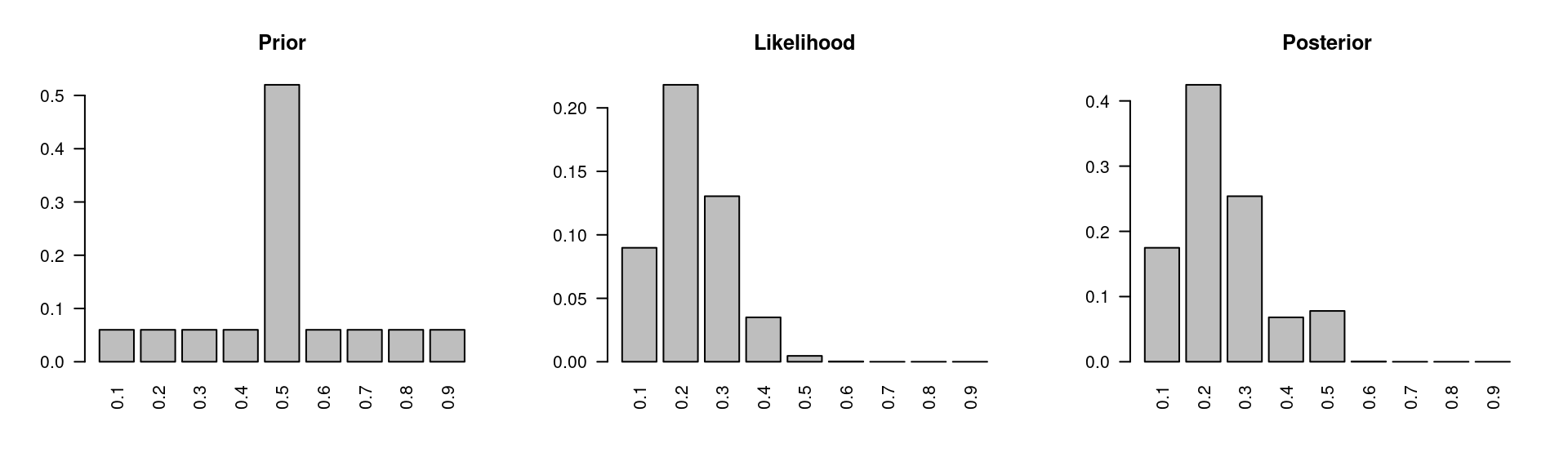
Figure 1.1: Original: sample size \(n=20\) and number of successes \(k=4\)
We started with the high prior at \(p=0.5\), but the data likelihood peaks at \(p=0.2\). And we updated our prior based on observed data to find the posterior. The Bayesian paradigm, unlike the frequentist approach, allows us to make direct probability statements about our models. For example, we can calculate the probability that RU-486, the treatment, is more effective than the control as the sum of the posteriors of the models where \(p<0.5\). Adding up the relevant posterior probabilities in Table 1.2, we get the chance that the treatment is more effective than the control is 92.16%.
1.2.3 Effect of Sample Size on the Posterior
The RU-486 example is summarized in Figure 1.1, and let’s look at what the posterior distribution would look like if we had more data.
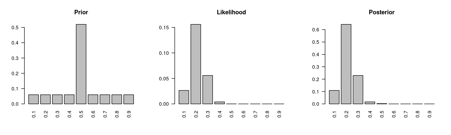
Figure 1.2: More data: sample size \(n=40\) and number of successes \(k=8\)
Suppose our sample size was 40 instead of 20, and the number of successes was 8 instead of 4. Note that the ratio between the sample size and the number of successes is still 20%. We will start with the same prior distribution. Then calculate the likelihood of the data which is also centered at 0.20, but is less variable than the original likelihood we had with the smaller sample size. And finally put these two together to obtain the posterior distribution. The posterior also has a peak at p is equal to 0.20, but the peak is taller, as shown in Figure 1.2. In other words, there is more mass on that model, and less on the others.
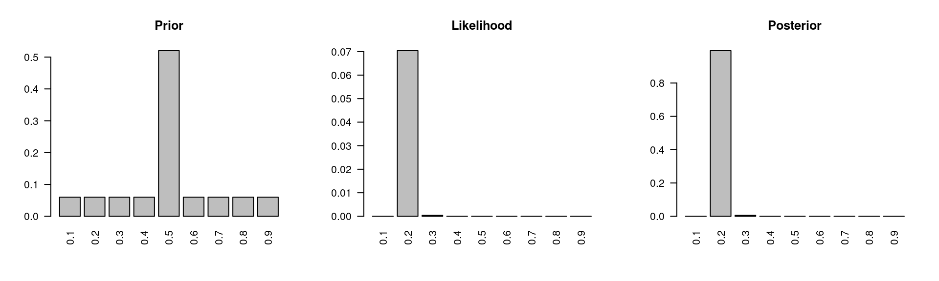
Figure 1.3: More data: sample size \(n=200\) and number of successes \(k=40\)
To illustrate the effect of the sample size even further, we are going to keep increasing our sample size, but still maintain the the 20% ratio between the sample size and the number of successes. So let’s consider a sample with 200 observations and 40 successes. Once again, we are going to use the same prior and the likelihood is again centered at 20% and almost all of the probability mass in the posterior is at p is equal to 0.20. The other models do not have zero probability mass, but they’re posterior probabilities are very close to zero.
Figure 1.3 demonstrates that as more data are collected, the likelihood ends up dominating the prior. This is why, while a good prior helps, a bad prior can be overcome with a large sample. However, it’s important to note that this will only work as long as we do not place a zero probability mass on any of the models in the prior.
1.3 Frequentist vs. Bayesian Inference
1.3.1 Frequentist vs. Bayesian Inference
In this section, we will solve a simple inference problem using both frequentist and Bayesian approaches. Then we will compare our results based on decisions based on the two methods, to see whether we get the same answer or not. If we do not, we will discuss why that happens.
Example 1.9 We have a population of M&M’s, and in this population the percentage of yellow M&M’s is either 10% or 20%. You have been hired as a statistical consultant to decide whether the true percentage of yellow M&M’s is 10% or 20%.
Payoffs/losses: You are being asked to make a decision, and there are associated payoff/losses that you should consider. If you make the correct decision, your boss gives you a bonus. On the other hand, if you make the wrong decision, you lose your job.
Data: You can “buy” a random sample from the population – You pay $200 for each M&M, and you must buy in $1,000 increments (5 M&Ms at a time). You have a total of $4,000 to spend, i.e., you may buy 5, 10, 15, or 20 M&Ms.
Remark: Remember that the cost of making a wrong decision is high, so you want to be fairly confident of your decision. At the same time, though, data collection is also costly, so you don’t want to pay for a sample larger than you need. If you believe that you could actually make a correct decision using a smaller sample size, you might choose to do so and save money and resources.
Let’s start with the frequentist inference.
Hypothesis: \(H_0\) is 10% yellow M&Ms, and \(H_A\) is >10% yellow M&Ms.
Significance level: \(\alpha = 0.05\).
One sample: red, green, yellow, blue, orange
Observed data: \(k=1, n=5\)
P-value: \(P(k \geq 1 | n=5, p=0.10) = 1 - P(k=0 | n=5, p=0.10) = 1 - 0.90^5 \approx 0.41\)
Note that the p-value is the probability of observed or more extreme outcome given that the null hypothesis is true.
Therefore, we fail to reject \(H_0\) and conclude that the data do not provide convincing evidence that the proportion of yellow M&M’s is greater than 10%. This means that if we had to pick between 10% and 20% for the proportion of M&M’s, even though this hypothesis testing procedure does not actually confirm the null hypothesis, we would likely stick with 10% since we couldn’t find evidence that the proportion of yellow M&M’s is greater than 10%.
The Bayesian inference works differently as below.
Hypotheses: \(H_1\) is 10% yellow M&Ms, and \(H_2\) is 20% yellow M&Ms.
Prior: \(P(H_1) = P(H_2) = 0.5\)
Sample: red, green, yellow, blue, orange
Observed data: \(k=1, n=5\)
Likelihood:
\[\begin{aligned} P(k=1 | H_1) &= \left( \begin{array}{c} 5 \\ 1 \end{array} \right) \times 0.10 \times 0.90^4 \approx 0.33 \\ P(k=1 | H_2) &= \left( \begin{array}{c} 5 \\ 1 \end{array} \right) \times 0.20 \times 0.80^4 \approx 0.41 \end{aligned}\]
- Posterior
\[\begin{aligned} P(H_1 | k=1) &= \frac{P(H_1)P(k=1 | H_1)}{P(k=1)} = \frac{0.5 \times 0.33}{0.5 \times 0.33 + 0.5 \times 0.41} \approx 0.45 \\ P(H_2 | k=1) &= 1 - 0.45 = 0.55 \end{aligned}\]
The posterior probabilities of whether \(H_1\) or \(H_2\) is correct are close to each other. As a result, with equal priors and a low sample size, it is difficult to make a decision with a strong confidence, given the observed data. However, \(H_2\) has a higher posterior probability than \(H_1\), so if we had to make a decision at this point, we should pick \(H_2\), i.e., the proportion of yellow M&Ms is 20%. Note that this decision contradicts with the decision based on the frequentist approach.
Table 1.3 summarizes what the results would look like if we had chosen larger sample sizes. Under each of these scenarios, the frequentist method yields a higher p-value than our significance level, so we would fail to reject the null hypothesis with any of these samples. On the other hand, the Bayesian method always yields a higher posterior for the second model where \(p\) is equal to 0.20. So the decisions that we would make are contradictory to each other.
| Frequentist | Bayesian H_1 | Bayesian H_2 | |
|---|---|---|---|
| Observed Data | P(k or more | 10% yellow) | P(10% yellow | n, k) | P(20% yellow | n, k) |
| n = 5, k = 1 | 0.41 | 0.45 | 0.55 |
| n = 10, k = 2 | 0.26 | 0.39 | 0.61 |
| n = 15, k = 3 | 0.18 | 0.34 | 0.66 |
| n = 20, k = 4 | 0.13 | 0.29 | 0.71 |
However, if we had set up our framework differently in the frequentist method and set our null hypothesis to be \(p = 0.20\) and our alternative to be \(p < 0.20\), we would obtain different results. This shows that the frequentist method is highly sensitive to the null hypothesis, while in the Bayesian method, our results would be the same regardless of which order we evaluate our models.
1.4 Exercises
Conditioning on dating site usage. Recall Table 1.1. What is the probability that an online dating site user from this sample is 18-29 years old?
Probability of no HIV. Consider the ELISA test from Section 1.1.2. What is the probability that someone has no HIV if that person has a negative ELISA result? How does this compare to the probability of having no HIV before any test was done?
Probability of no HIV after contradictive tests. Consider the ELISA test from Section 1.1.2. What is the probability that someone has no HIV if that person first tests positive on the ELISA and secondly test negative? Assume that the tests are independent from each other.